Google Sheets

Formula Hot Sheet
Google Sheets How-To
Google Sheets - Super Menu w/ Apps Script

Formula Hot Sheet

Formula HotSheet

I’ve been using Excel / Google Sheets since 2002 or so. This isn’t a breakdown of the basics, but rather, a place where I dump more complex formulas for reference later.

Some Low-Hanging-Fruit

Here’s a formula that tells you what the date is today

=today()

Here’s a formula that calculates the days between two dates (where E5 is date 1, and E4 is date 2)

=DAYS(E5,E4)

Here’s a that will concat a separate date & time field, and keep it formatted as you desire

=TEXT(B12, "M/DD/YYYY")&" "&TEXT(C12, "h:mmam/pm")

Concatenating more than one date and/or time requires using the TEXT function, otherwise you’ll end up with numbers that don’t mean anything to you.

Timecode

These formulas will take 00:00:00:00 formatted timecode 30fps or 60fps timecode and convert it to frame count (where cell B5 = timecode) or perform calculations or convert from frame count back to formatted timecode. Note, these only work for WHOLE FRAME timecode (eg, 23.976 won’t work).

30fps

=SUM(SUM(SUM(MID(B5, 4,2)*60)+SUM(MID(B5,7,2)*1))*30,N("FPS"))+SUM(RIGHT(B5,2)*1)

Where B2 = FPS cell and A2:A is a range of timecode to add -

=SUMPRODUCT(IFERROR(SPLIT(A2:A,":")*{B2*3600,B2*60,B2,1}))

60fps

=SUM(SUM(SUM(MID(B5, 4,2)*60)+SUM(MID(B5,7,2)*1))*60,N("FPS"))+SUM(RIGHT(B5,2)*1)

Where B2 = FPS cell and A2:A is a range of timecode to add -

=SUMPRODUCT(IFERROR(SPLIT(A2:A,":")*{B2*3600,B2*60,B2,1}))

Converting Frame Count Duration (eg "156")

Into formatted timecode. Where C2 = total frame count and B2 = FPS

=TEXT(TIME(0,0,C2/B2),"hh:mm:ss") &":"& TEXT(MOD(C2,B2),"00")

Performing a Timecode Calculation

from formatted timecode (math happens over frame counts), then converting it back to proper timecode format. Where B2 = FPS, A2:A = Range

=TEXT(TIME(0,0,SUMPRODUCT(
    IFERROR(SPLIT(A2:A,":")*{B2*3600,B2*60,B2,1})
  )/B2),"hh:mm:ss")
  &":"&TEXT(MOD(SUMPRODUCT(RIGHT(A2:A,2)),B2),"00")

Automatic Population Based on IF

Here’s a formula that will automatically populate a cell with whatever’s furthest to the right in a column (from column C through column ZZ, row 4)

=ArrayFormula((IFERROR(LOOKUP( 2, 1 / ( C4:ZZ4 <> "" ), C4:ZZ4 ),"")))

Here’s a formula that will automatically populate a cell with a most recent date from a header row if the array’s data row contains text. The 5th row is the date row. The 7th row is the data row.

=ArrayFormula(IFERROR(LOOKUP(2,1/(G7:Z7>0),$G$5:$Z$5),"None"))

Conditional Formatting

Oddly, you need to apply absolute cell references (either column or row, depending on formula goal) if you want conditional formatting to copy and paste and stay relational, you apply the absolute technique. This will keep things relational in a conditional formatting copy/paste.

This will apply conditional formatting if the referenced cell (A1) contains the word “Cat”. Literally, if A1 contains “Cat”, then toggle on, else toggle off:

=if(regexmatch($A1,"Cat"),1,0)

This will apply conditional formatting if the referenced cell (A1) contains the word “someword” where “someword” is case sensitive

=if(REGEXMATCH($A1,"(?i).*someword.*"),1,0)

This will apply conditional formatting in a cell if the reference cell is checked (using the inserted checkbox function). In this example, this applied in cell E7. So if D7 is checked, E7 will follow the conditional formatting rule.

=IF($D7,1,0)

=IF($D7,1,0)

This will do the exact same thing, with different syntax:

=$D7=TRUE

This set of conditional format will apply based on the number of days ago, where $E7 represents the target cell (self). This conditional format can be copied and applied to a range without changing the formula. The first time you put it in it needs to refer to the correct cell, but then will work from there.

Applies conditional formatting if the current cell date is between 0 and 6 days ago

=IF((((DAYS($E7, TODAY()))>=-6)*((DAYS($E7, TODAY()))<=0))=1,1,0)

Applies conditional formatting if the current cell date is between 7 and 13 days ago

=IF((((DAYS($E7, TODAY()))>=-13)*((DAYS($E7, TODAY()))<=-7))=1,1,0)

Applies conditional formatting if the current cell date is between 14 and 20 days ago

=IF((((DAYS($E7, TODAY()))>=-20)*((DAYS($E7, TODAY()))<=-14))=1,1,0)

Applies conditional formatting if the current cell date is more than 20 days ago

=IF(DAYS($E7, TODAY())<-21,1,0)

This will apply conditional formatting to the most recent date as a header row. The first cell reference here has to be the first cell in the range (eg G5) and it applies to all of row 5.

=G5=MAX($5:$5)

Google Sheets How-To

Need Leading Zeros?

Set number format to “custom number format” and enter the number of zeros for the number of digits you need. For example, a custom number format of “00” will turn “1” into “01” and “14” will just stay “14”. You can also this in formula by saying =TEXT(SomeCell,”0000”). If some Cell is B6 and B6 = 16, than that formula will return 0016.

Need Unique Row IDs?

This took a surprising amount of effort.

If you’ve got a note tracker or just need to create unique IDs for rows that persist through a sort or a filter or an insert of rows, and you don’t it to get all wonky, follow the steps below

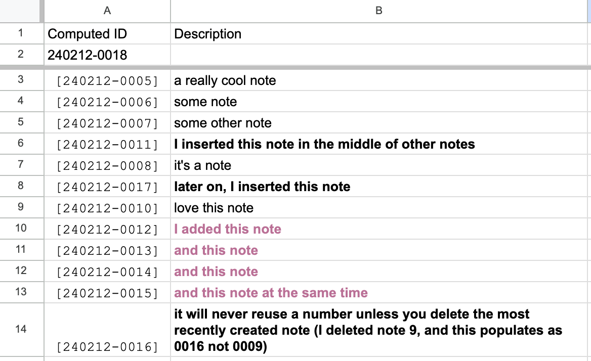First, put a head in A1 called “Computed IDs”, then put a formula in A2 that counts all of the existing IDs and then adds ONE. It’s looking for the last portion of an ID string that is always the same number of digits (alpha/numeric). The first note would come with an ID that looks like this: [240212-0001] You’ll need to populate one row with the first ID for the formula to work from there.

Here’s the formula to put in A2

=TEXT(TODAY(),"YYMMDD")&"-"&TEXT((MAX(ArrayFormula(VALUE(MID(A3:A,9,4))))+1),"0000")

It is recommended that you delete all unused rows before you proceed to next steps, otherwise you’ll generate 1000 ids on blank rows.

Second, in Apps Script (Extensions→Apps Script) create a new script called MakeIDs.gs

This script will print whatever’s in cell A2 down all of column A. It will never repeat a number or replace an existing ID. It does this through a LOOP, so it does one empty row, then another, etc. The only time it will reuse a number is when you delete the last renaming number (because it no longer exists, it doesn’t know that it used to exist).

It will put that value in brackets. You can change that very easily to be in a different cell or remove the brackets entirely.

function MakeIDs() {
  var sheet = SpreadsheetApp.getActiveSpreadsheet().getActiveSheet();
  var valueToCopy = "[" + sheet.getRange("A2").getValue() + "]"; // Adding "[" at the beginning and "]" at the end
  var columnAValues = sheet.getRange("A3:A").getValues(); // Adjusted range to start from A3
  
  var i = 0;
  while (i < columnAValues.length) {
    if (columnAValues[i][0] === "") {
      sheet.getRange(i + 3, 1).setValue(valueToCopy); // Adjusted row index to match starting row
      break; // Exit loop after copying to the first empty cell in column A
    }
    i++;
  }
  
  if (i === columnAValues.length) {
    // All cells in column A are populated, stop the function
    return;
  } else {
    // Call the function recursively to continue copying until all cells are populated
    MakeIDs();
  }
}

Third

You want to create a way to run this command, so create another script in Apps Script called “FillMenu” (you can change ‘CustomMenu’ to whatever name you want).

function onOpen() {
   var spreadsheet = SpreadsheetApp.getActive();
   var menuItems = [
     {name: 'Make IDs', functionName: 'MakeIDs'},
   ];
   spreadsheet.addMenu('CustomMenu', menuItems);
}

Now, refresh the Google Sheet in your web browser and a new menu item will come up called CustomMenu and a command called MakeIDs. Run it and watch your cells populate with new numbers. Add more rows, click it again. Huzzah!

Google Sheets - Super Menu w/ Apps Script

Add a sweet fuckin' menu in Google Sheets that will shave off hours of your life. After all, time is the only resource you can never get back.

Replace fill color (replaceFillColor) - Finds all cells with hex color and replaces the hex color of your choosing
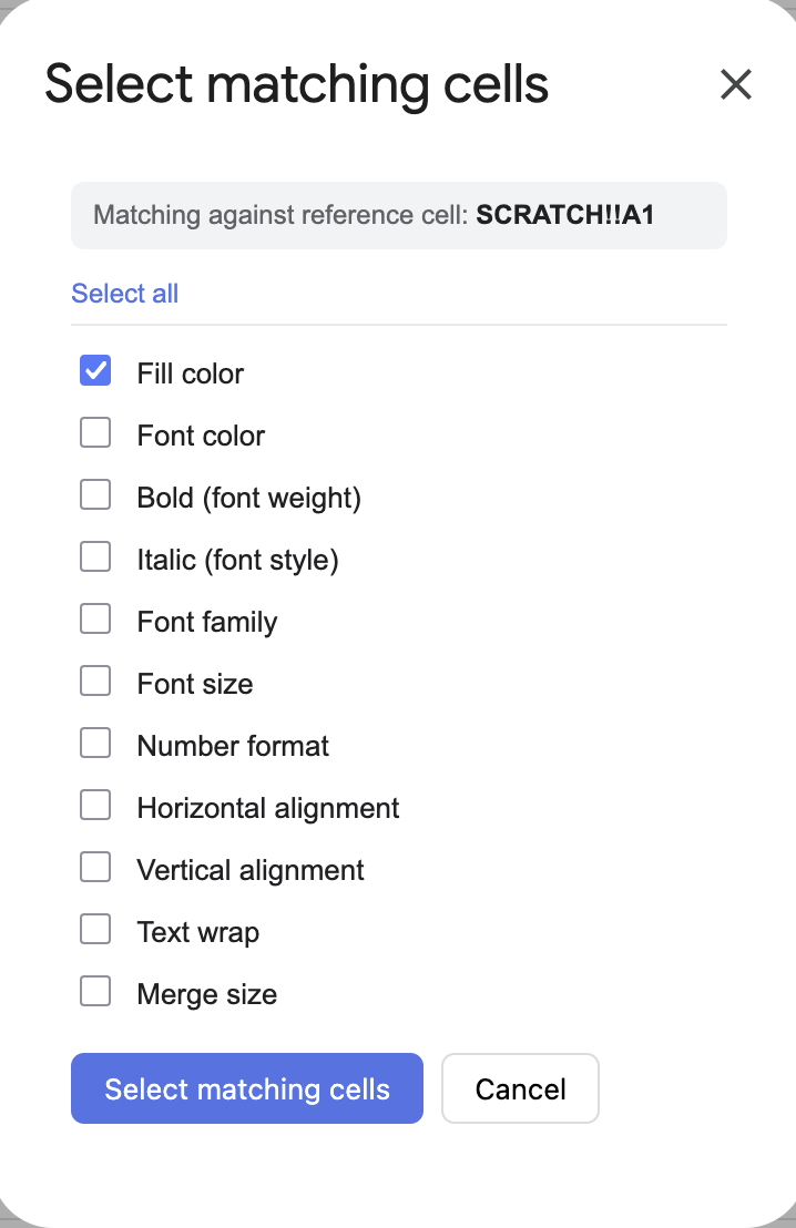
Select matching cells (selectMatchingCells) - This one is so tight, you can find all cells that match certain conditions and bulk edit them.
Copy (Formula Safe) - this copies formats and formulas of a selection
Paste (Formula Safe) - this copies formats and formulas of a selection, formulas references are absolute and aren't transposed (unless they are referenced within the copied selection, and then the self-reference updates). You're welcome!!!

Here's the Apps Script

/**
 * Tech Almanac Tools — utilities under a sub menu:
 *   1. Replace fill color   (replaceFillColor)
 *   2. Select matching cells (selectMatchingCells)
 *   3. Copy (Formula Safe) - this copies formats and formulas of a selection
 *   4. Paste (Formula Safe) - this copies formats and formulas of a selection, formulas references are absolute and aren't transposed (unless they are referenced within the copied selection, and then the self-reference updates). You're welcome!!!
 * "Select matching cells" needs a companion HTML file named "MatchDialog".
 */

function onOpen() {
  SpreadsheetApp.getUi()
    .createMenu('Tech Almanac Tools')
    .addItem('Replace fill color…', 'replaceFillColor')
    .addItem('Select matching cells…', 'selectMatchingCells')
    .addSeparator()
    .addItem('Copy (formula-safe)', 'formulaSafeCopy')
    .addItem('Paste (formula-safe)', 'formulaSafePaste')
    .addToUi();
}

/* ============================================================
 * TOOL 1 — Replace fill color
 * ============================================================ */

function replaceFillColor() {
  const ui = SpreadsheetApp.getUi();
  const sheet = SpreadsheetApp.getActiveSheet();

  const findResp = ui.prompt(
    'Replace fill color',
    'Color to FIND (hex, e.g. #cfecff):',
    ui.ButtonSet.OK_CANCEL
  );
  if (findResp.getSelectedButton() !== ui.Button.OK) return;
  const findColor = normalizeHex(findResp.getResponseText());
  if (!findColor) {
    ui.alert('That doesn\'t look like a valid hex color. Try something like #cfecff.');
    return;
  }

  const replaceResp = ui.prompt(
    'Replace fill color',
    'Color to REPLACE it with (hex, e.g. #ffffff):',
    ui.ButtonSet.OK_CANCEL
  );
  if (replaceResp.getSelectedButton() !== ui.Button.OK) return;
  const replaceColor = normalizeHex(replaceResp.getResponseText());
  if (!replaceColor) {
    ui.alert('That doesn\'t look like a valid hex color. Try something like #ffffff.');
    return;
  }

  const range = sheet.getDataRange();
  const backgrounds = range.getBackgrounds();
  const startRow = range.getRow();
  const startCol = range.getColumn();

  const matchedA1 = [];
  for (let r = 0; r < backgrounds.length; r++) {
    for (let c = 0; c < backgrounds[r].length; c++) {
      if (backgrounds[r][c].toLowerCase() === findColor) {
        backgrounds[r][c] = replaceColor;
        matchedA1.push(sheet.getRange(startRow + r, startCol + c).getA1Notation());
      }
    }
  }

  if (matchedA1.length === 0) {
    ui.alert('No cells with fill ' + findColor + ' found on "' + sheet.getName() + '".');
    return;
  }

  sheet.setActiveRangeList(sheet.getRangeList(matchedA1));

  const confirm = ui.alert(
    'Confirm replacement',
    'Found ' + matchedA1.length + ' cell(s) with ' + findColor +
    ' on "' + sheet.getName() + '".\n\nReplace their fill with ' + replaceColor + '?',
    ui.ButtonSet.OK_CANCEL
  );
  if (confirm !== ui.Button.OK) return;

  range.setBackgrounds(backgrounds);
  SpreadsheetApp.getActive().toast('Replaced ' + matchedA1.length + ' cell(s).', 'Done', 5);
}

/**
 * Normalize a user-entered hex string to lowercase 6-digit form (#rrggbb).
 * Accepts "#cfecff", "cfecff", "#abc", "abc". Returns null if invalid.
 */
function normalizeHex(input) {
  if (!input) return null;
  let h = input.trim().toLowerCase().replace(/^#/, '');
  if (/^[0-9a-f]{3}$/.test(h)) {
    h = h.split('').map(function (ch) { return ch + ch; }).join('');
  }
  if (/^[0-9a-f]{6}$/.test(h)) return '#' + h;
  return null;
}

/* ============================================================
 * TOOL 2 — Select matching cells
 * ============================================================ */

function selectMatchingCells() {
  const html = HtmlService.createHtmlOutputFromFile('MatchDialog')
    .setWidth(320)
    .setHeight(460);
  SpreadsheetApp.getUi().showModalDialog(html, 'Select matching cells');
}

/** Called by the dialog on load, to show which cell is the reference. */
function getActiveCellAddress() {
  const sheet = SpreadsheetApp.getActiveSheet();
  return sheet.getName() + '!' + sheet.getActiveCell().getA1Notation();
}

/**
 * Called by the dialog. `options` is an object of booleans keyed by attribute.
 * Selects every cell on the active sheet that matches the reference cell on
 * all enabled attributes. Returns { count } or { error }.
 */
function runMatch(options) {
  const sheet = SpreadsheetApp.getActiveSheet();
  const range = sheet.getDataRange();
  const startRow = range.getRow();
  const startCol = range.getColumn();
  const numRows = range.getNumRows();
  const numCols = range.getNumColumns();

  // Reference cell position relative to the data range.
  const active = sheet.getActiveCell();
  let refR = active.getRow() - startRow;
  let refC = active.getColumn() - startCol;
  if (refR < 0 || refC < 0 || refR >= numRows || refC >= numCols) {
    return { error: 'Select a cell that contains data first, then run this again.' };
  }

  // Read only the attribute matrices we actually need.
  const data = {};
  if (options.background)   data.background   = range.getBackgrounds();
  if (options.fontColor)    data.fontColor    = range.getFontColors();
  if (options.fontWeight)   data.fontWeight   = range.getFontWeights();
  if (options.fontStyle)    data.fontStyle    = range.getFontStyles();
  if (options.fontFamily)   data.fontFamily   = range.getFontFamilies();
  if (options.fontSize)     data.fontSize     = range.getFontSizes();
  if (options.numberFormat) data.numberFormat = range.getNumberFormats();
  if (options.hAlign)       data.hAlign       = range.getHorizontalAlignments();
  if (options.vAlign)       data.vAlign       = range.getVerticalAlignments();
  if (options.wrap)         data.wrap         = range.getWraps();

  const hasAttr = Object.keys(data).length > 0;
  if (!hasAttr && !options.merge) {
    return { error: 'Pick at least one condition to match on.' };
  }

  // Build merge maps: dimensions string per cell + which cells are anchors.
  const mergeDims = [];
  const isAnchor = [];
  for (let r = 0; r < numRows; r++) {
    mergeDims[r] = new Array(numCols).fill('1x1');
    isAnchor[r] = new Array(numCols).fill(true);
  }
  const merges = range.getMergedRanges();
  merges.forEach(function (m) {
    const mr = m.getRow() - startRow;
    const mc = m.getColumn() - startCol;
    const rows = m.getNumRows();
    const cols = m.getNumColumns();
    const dim = rows + 'x' + cols;
    for (let r = mr; r < mr + rows; r++) {
      for (let c = mc; c < mc + cols; c++) {
        if (r >= 0 && c >= 0 && r < numRows && c < numCols) {
          mergeDims[r][c] = dim;
          isAnchor[r][c] = (r === mr && c === mc);
        }
      }
    }
    // Snap the reference to its merge anchor if it sits inside this merge.
    if (refR >= mr && refR < mr + rows && refC >= mc && refC < mc + cols) {
      refR = mr;
      refC = mc;
    }
  });

  // Reference values.
  const ref = {};
  Object.keys(data).forEach(function (k) {
    ref[k] = norm(k, data[k][refR][refC]);
  });
  const refMerge = mergeDims[refR][refC];

  // Scan and collect anchor cells that match on every enabled attribute.
  const matched = [];
  for (let r = 0; r < numRows; r++) {
    for (let c = 0; c < numCols; c++) {
      if (!isAnchor[r][c]) continue; // skip interior cells of merges
      let ok = true;
      for (const k in data) {
        if (norm(k, data[k][r][c]) !== ref[k]) { ok = false; break; }
      }
      if (ok && options.merge && mergeDims[r][c] !== refMerge) ok = false;
      if (ok) matched.push(sheet.getRange(startRow + r, startCol + c).getA1Notation());
    }
  }

  if (matched.length === 0) return { count: 0 };
  sheet.setActiveRangeList(sheet.getRangeList(matched));
  return { count: matched.length };
}

/** Normalize values so equivalent formats compare equal (colors are case-folded). */
function norm(key, val) {
  if (key === 'background' || key === 'fontColor') return String(val).toLowerCase();
  return val;
}

// ── Formula-Safe Copy ────────────────────────────────────────────────────────

function formulaSafeCopy() {
  const sheet = SpreadsheetApp.getActiveSpreadsheet().getActiveSheet();
  const range = sheet.getActiveRange();

  // Store the A1 notation and sheet name in script properties
  const props = PropertiesService.getScriptProperties();
  props.setProperty('FSC_RANGE',  range.getA1Notation());
  props.setProperty('FSC_SHEET',  sheet.getName());

  SpreadsheetApp.getUi().alert(
    `Copied ${range.getA1Notation()} — now select your destination cell and run Paste (formula-safe).`
  );
}

// ── Formula-Safe Paste ───────────────────────────────────────────────────────

function formulaSafePaste() {
  const ui    = SpreadsheetApp.getUi();
  const props = PropertiesService.getScriptProperties();
  const srcRangeNotation = props.getProperty('FSC_RANGE');
  const srcSheetName     = props.getProperty('FSC_SHEET');

  if (!srcRangeNotation || !srcSheetName) {
    ui.alert('Nothing copied yet — run Copy (formula-safe) first.');
    return;
  }

  const ss       = SpreadsheetApp.getActiveSpreadsheet();
  const srcSheet = ss.getSheetByName(srcSheetName);
  const srcRange = srcSheet.getRange(srcRangeNotation);

  // Grab formulas (as strings) and display values separately
  const formulas = srcRange.getFormulas();       // raw formula strings, e.g. "=A1+B1"
  const values   = srcRange.getDisplayValues();  // what the cell shows if not a formula

  // Source range bounds
  const srcRow  = srcRange.getRow();
  const srcCol  = srcRange.getColumn();
  const srcRows = srcRange.getNumRows();
  const srcCols = srcRange.getNumColumns();

  // Destination anchor
  const dest    = ss.getActiveSheet().getActiveRange();
  const destRow = dest.getRow();
  const destCol = dest.getColumn();

  // Row/col offset from source to destination
  const rowOffset = destRow - srcRow;
  const colOffset = destCol - srcCol;

  // Regex matches cell addresses like B4, $B$4, B$4, $B4
  const cellRef = /(\$?)([A-Za-z]{1,3})(\$?)(\d+)/g;

  /**
   * If the address falls within the source range, shift it by the paste offset.
   * Anchored ($) axes are never shifted, matching normal paste behaviour.
   * Addresses outside the source range are left untouched.
   */
  function shiftIfInRange(colAnchor, colLetter, rowAnchor, rowNum) {
    const col = columnLetterToIndex(colLetter.toUpperCase());
    const row = parseInt(rowNum, 10);
    if (row >= srcRow && row < srcRow + srcRows &&
        col >= srcCol && col < srcCol + srcCols) {
      const newCol = colAnchor ? col : col + colOffset;
      const newRow = rowAnchor ? row : row + rowOffset;
      return (colAnchor ? '$' : '') + columnIndexToLetter(newCol) +
             (rowAnchor ? '$' : '') + newRow;
    }
    return (colAnchor ? '$' : '') + colLetter.toUpperCase() +
           (rowAnchor ? '$' : '') + rowNum;
  }

  // Build payload: rewrite intra-range references, pass external refs through as-is
  const payload = formulas.map((row, r) =>
    row.map((formula, c) => {
      if (formula === '') return values[r][c];
      return formula.replace(cellRef, (match, ca, cl, ra, rn) =>
        shiftIfInRange(ca, cl, ra, rn)
      );
    })
  );

  const destRange = ss.getActiveSheet().getRange(
    destRow, destCol, payload.length, payload[0].length
  );

  // Copy formatting first, then overwrite with values/formulas
  srcRange.copyTo(destRange, SpreadsheetApp.CopyPasteType.PASTE_FORMAT, false);
  destRange.setValues(payload);
}

// ── Helpers ──────────────────────────────────────────────────────────────────

function columnLetterToIndex(letters) {
  let n = 0;
  for (let i = 0; i < letters.length; i++) {
    n = n * 26 + (letters.charCodeAt(i) - 64);
  }
  return n;
}

function columnIndexToLetter(n) {
  let s = '';
  while (n > 0) {
    const rem = (n - 1) % 26;
    s = String.fromCharCode(65 + rem) + s;
    n = Math.floor((n - 1) / 26);
  }
  return s;
}

Here's the MarchDialog.html for the Select Matching Cells Modal

<!DOCTYPE html>
<html>
<head>
  <base target="_top">
  <style>
    body {
      font-family: Arial, Helvetica, sans-serif;
      font-size: 13px;
      color: #202124;
      margin: 12px;
    }
    .ref {
      background: #f1f3f4;
      border-radius: 6px;
      padding: 8px 10px;
      margin-bottom: 12px;
      font-size: 12px;
      color: #5f6368;
    }
    .ref b { color: #202124; }
    label {
      display: block;
      padding: 4px 0;
      cursor: pointer;
    }
    label input { margin-right: 8px; }
    .toggle {
      margin-bottom: 6px;
      padding-bottom: 6px;
      border-bottom: 1px solid #e8eaed;
    }
    .toggle a {
      font-size: 12px;
      color: #1a73e8;
      text-decoration: none;
      cursor: pointer;
    }
    .toggle a:hover { text-decoration: underline; }
    .buttons {
      margin-top: 14px;
      display: flex;
      gap: 8px;
    }
    button {
      font-size: 13px;
      padding: 7px 14px;
      border-radius: 6px;
      border: 1px solid #dadce0;
      background: #fff;
      cursor: pointer;
    }
    button.primary {
      background: #1a73e8;
      color: #fff;
      border-color: #1a73e8;
    }
    button:disabled { opacity: 0.5; cursor: default; }
    #status { margin-top: 12px; font-size: 12px; min-height: 16px; }
    #status.err { color: #c5221f; }
    #status.ok { color: #188038; }
  </style>
</head>
<body>
  <div class="ref">
    Matching against reference cell: <b id="refCell">…</b>
  </div>

  <div class="toggle">
    <a href="#" id="toggleAll" onclick="toggleAll(); return false;">Select all</a>
  </div>

  <div id="opts">
    <label><input type="checkbox" id="background" checked> Fill color</label>
    <label><input type="checkbox" id="fontColor"> Font color</label>
    <label><input type="checkbox" id="fontWeight"> Bold (font weight)</label>
    <label><input type="checkbox" id="fontStyle"> Italic (font style)</label>
    <label><input type="checkbox" id="fontFamily"> Font family</label>
    <label><input type="checkbox" id="fontSize"> Font size</label>
    <label><input type="checkbox" id="numberFormat"> Number format</label>
    <label><input type="checkbox" id="hAlign"> Horizontal alignment</label>
    <label><input type="checkbox" id="vAlign"> Vertical alignment</label>
    <label><input type="checkbox" id="wrap"> Text wrap</label>
    <label><input type="checkbox" id="merge"> Merge size</label>
  </div>

  <div class="buttons">
    <button class="primary" id="run" onclick="run()">Select matching cells</button>
    <button onclick="google.script.host.close()">Cancel</button>
  </div>

  <div id="status"></div>

  <script>
    var KEYS = ['background','fontColor','fontWeight','fontStyle','fontFamily',
                'fontSize','numberFormat','hAlign','vAlign','wrap','merge'];

    google.script.run.withSuccessHandler(function (addr) {
      document.getElementById('refCell').textContent = addr;
    }).getActiveCellAddress();

    function setStatus(msg, cls) {
      var s = document.getElementById('status');
      s.textContent = msg;
      s.className = cls || '';
    }

    function syncToggleLabel() {
      var allChecked = KEYS.every(function (k) {
        return document.getElementById(k).checked;
      });
      document.getElementById('toggleAll').textContent = allChecked ? 'Select none' : 'Select all';
    }
    KEYS.forEach(function (k) {
      document.getElementById(k).addEventListener('change', syncToggleLabel);
    });
    syncToggleLabel();

    function toggleAll() {
      var allChecked = KEYS.every(function (k) {
        return document.getElementById(k).checked;
      });
      KEYS.forEach(function (k) { document.getElementById(k).checked = !allChecked; });
      syncToggleLabel();
    }

    function run() {
      var options = {};
      KEYS.forEach(function (k) { options[k] = document.getElementById(k).checked; });

      var btn = document.getElementById('run');
      btn.disabled = true;
      setStatus('Scanning…');

      google.script.run
        .withSuccessHandler(function (result) {
          btn.disabled = false;
          if (result.error) { setStatus(result.error, 'err'); return; }
          if (result.count === 0) { setStatus('No matching cells found.', 'err'); return; }
          setStatus('Selected ' + result.count + ' cell(s). Closing…', 'ok');
          setTimeout(google.script.host.close, 700);
        })
        .withFailureHandler(function (err) {
          btn.disabled = false;
          setStatus(err.message || String(err), 'err');
        })
        .runMatch(options);
    }
  </script>
</body>
</html>