Google Sheets How-To

Need Leading Zeros? 

Set number format to “custom number format” and enter the number of zeros for the number of digits you need. For example, a custom number format of “00” will turn “1” into “01” and “14” will just stay “14”. You can also this in formula by saying =TEXT(SomeCell,”0000”). If some Cell is B6 and B6 = 16, than that formula will return 0016. 

Need Unique Row IDs?

This took a surprising amount of effort.   If you’ve got a note tracker or just need to create unique IDs for rows that persist through a sort or a filter or an insert of rows, and you don’t it to get all wonky, follow the steps below

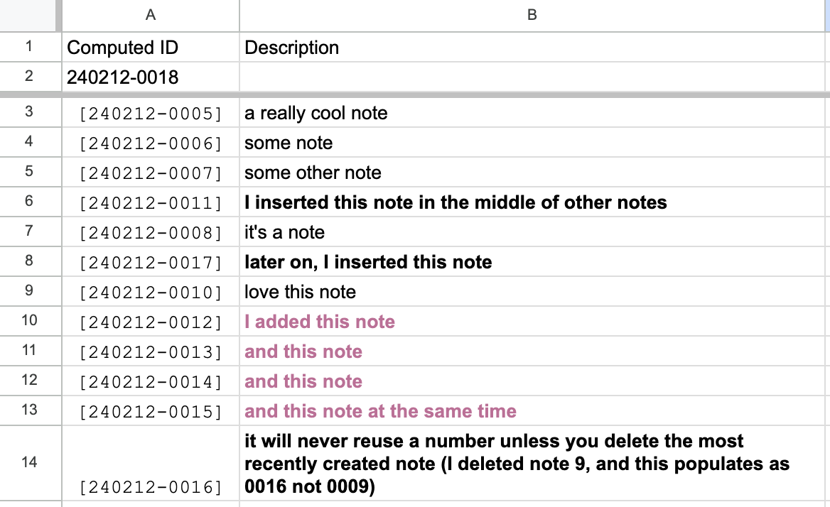First, put a head in A1 called “Computed IDs”, then put a formula in A2 that counts all of the existing IDs and then adds ONE. It’s looking for the last portion of an ID string that is always the same number of digits (alpha/numeric). The first note would come with an ID that looks like this: [240212-0001] You’ll need to populate one row with the first ID for the formula to work from there. 

Here’s the formula to put in A2

=TEXT(TODAY(),"YYMMDD")&"-"&TEXT((MAX(ArrayFormula(VALUE(MID(A3:A,9,4))))+1),"0000")

It is recommended that you delete all unused rows before you proceed to next steps, otherwise you’ll generate 1000 ids on blank rows. 

Second, in Apps Script (Extensions→Apps Script) create a new script called MakeIDs.gs

This script will print whatever’s in cell A2 down all of column A. It will never repeat a number or replace an existing ID. It does this through a LOOP, so it does one empty row, then another, etc. The only time it will reuse a number is when you delete the last renaming number (because it no longer exists, it doesn’t know that it used to exist). 

It will put that value in brackets. You can change that very easily to be in a different cell or remove the brackets entirely. 

function MakeIDs() {
  var sheet = SpreadsheetApp.getActiveSpreadsheet().getActiveSheet();
  var valueToCopy = "[" + sheet.getRange("A2").getValue() + "]"; // Adding "[" at the beginning and "]" at the end
  var columnAValues = sheet.getRange("A3:A").getValues(); // Adjusted range to start from A3
  
  var i = 0;
  while (i < columnAValues.length) {
    if (columnAValues[i][0] === "") {
      sheet.getRange(i + 3, 1).setValue(valueToCopy); // Adjusted row index to match starting row
      break; // Exit loop after copying to the first empty cell in column A
    }
    i++;
  }
  
  if (i === columnAValues.length) {
    // All cells in column A are populated, stop the function
    return;
  } else {
    // Call the function recursively to continue copying until all cells are populated
    MakeIDs();
  }
}

Third

You want to create a way to run this command, so create another script in Apps Script called “FillMenu” (you can change ‘CustomMenu’ to whatever name you want). 

function onOpen() {
   var spreadsheet = SpreadsheetApp.getActive();
   var menuItems = [
     {name: 'Make IDs', functionName: 'MakeIDs'},
   ];
   spreadsheet.addMenu('CustomMenu', menuItems);
}

Now, refresh the Google Sheet in your web browser and a new menu item will come up called CustomMenu and a command called MakeIDs. Run it and watch your cells populate with new numbers. Add more rows, click it again. Huzzah!